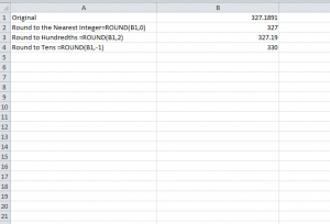
The ROUND Function is the best way to get your data looking just the way you want it. This simple formula takes any decimal figures and simply rounds that number, or number set, to whatever decimal place you need. It can be tedious to go through a large list of numbers and enter the decimal place you want for each calculation. You could have pages and pages of numbers that need to be corrected, wasting your time and energy in the process. Instead, you can use this handy feature to quickly and efficiently create the desired look for your document.
How to Use ROUND Functions in Your Spreadsheet
There are a number of different rounding formulas you can use to get your spreadsheet looking nice and neat. However, it’s best to first understand the fundamental structure of this type of function. Generally, the function will be written =ROUND(X,Y). X in this context represents the original value or cell you want to change and Y representing the number of digits you want to round to.
As an example, you can have the function “=ROUND(555.66666,2),” which will round your figure to “555.67.”
Similarly, you can use the ROUNDUP, ROUNDDOWN, and MROUND Functions for different things.
The ROUNDUP Function allows you to consistently round your figures up throughout the document, as the ROUNDDOWN Function will always round your numbers down the amount of your choosing.
The MROUND Function is intended to round figures to a specific decimal place, such as 25. To accomplish this, simply enter the same formula as with the ROUND function. However, X will now be the number rounded and Y is the multiple to round to.
The ROUND function makes your life easier by giving you a way to display your data just the way you want it.
Download: How to Use the ROUND Function in Excel
Check out this offer while you wait!

