The AVERAGE Top 4 Template is a great way to learn how to use a simple and effective Excel function to find the AVERAGEs for a set of data instantly. Once you download the free template below, this guide will show you step-by-step how to use the AVERAGE function to achieve the result you want. Whether you want to find the AVERAGEs of your favorite team’s scores or your need to keep track of your students AVERAGE grades, this template has the tools you need to add a simple function to your growing knowledge of everything Excel. Continue reading the guide below to get started.

How to Use the AVERAGE Top 4 Template

Once you have successfully downloaded the free template file to your computer by clicking the link at the bottom of this page, you are free to follow along with the guide below.

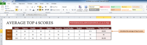
The template is pretty simple so you can learn how to use the function quickly. You will find a row of school subjects at the top of the page and the AVERAGE grades from the past three semesters for them in each column.

In the very last column of the template, the AVERAGE function will be applied to the data set to give you the information you need.

The general formula will look like this,

=AVERAGE(LARGE(range,{1,2,3,4}))

You simply have to enter your own data into the above formula to get the desired answer. Let’s say you want to calculate the AVERAGE grades of the first semester. Your new formula will look like this,

=AVERAGE(LARGE(C5:K5,{1,2,3,4}))

With this new formula, you will get the AVERAGE of the top 4 scores from C5 to K5 (the first row of the template). If you want to expand to the top 5, 6, 7, etc. scores you would just continue the pattern at the end of the formula and close the function the same way it is displayed in the two examples above.

Download: AVERAGE top 4 scores