

Excel’s Pivot Table function allows you to easily arrange and summarize large amounts of data to pull the details and view them.
Download the Pivot Table example to get started
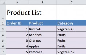
Begin by clicking a cell inside the pre-filled data area.
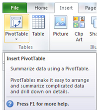
Click the “Insert” tab at the top and choose PivotTable from the options.
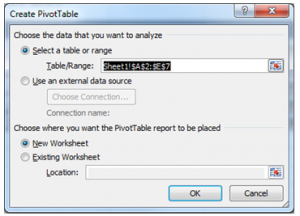
The “Create PivotTable” dialog box appears. It will tell you the range of the pivot table that will be created.
Choose whether you want the PivotTable to be in a new worksheet or the sheet you’re currently working on. Press OK once you’ve finished.
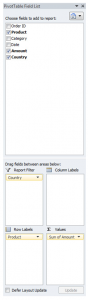
The field list will pop onto the screen. For this example, choose to add:
Product Field to Row Labels
Amount to Values area.
Country to Report Filters.
Your PivotTable has now been produced! It should look like this:
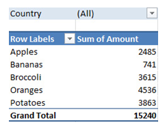
Use Excel’s Pivot Table function to arrange large amounts of data into easy to read fields.
Check out this offer while you wait!