The AUTOFILTER function is one of the best tools offered by Excel. Creating a table to house your information is an efficient way to organize your data. This function is also extremely helpful when you’re searching through your document for specific terms. Now you can track the progress of individuals, sales, products, and anything else you want to sort. All you need to do is click on the category you want to view, and the AUTOFILTER feature will temporarily remove all other categories in a single column instantly. Nothing can be simpler. Read the steps below to learn how it’s done.
Steps to Use the AUTOFILTER Function in Excel
You’ll need to create a list in the appropriate format to begin using the AUTOFILTER function. To view an example of the proper format for your table, simply click the link below to download the sample spreadsheet.
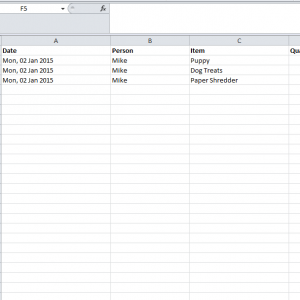
Notice how each category in the first row has its own AUTOFILTER drop-down menu. The basic format will be a row of categories at the top of the page and a list of items corresponding to each of these categories. To make things simple, the sample document only contains the sales information for two employees.
Once you have your table set up in a similar fashion to the example spreadsheet, you can use the AUTOFILTER function.
Highlight your category row at the top of your template. Then, click on the “Sort and Filter” button in the home ribbon to the right of your screen. A drop-down menu will appear under this button, choose the “Filter” option to create your AUTOFILTER menus.
When you go back to your categories at the top of the spreadsheet, you will see the AUTOFILTER drop-down menus displayed for each item.
Simply check the item you want to analyze and deselect all other options in the drop-down menu. This will temporarily remove all other items in that column, allowing you to focus on what you need. When you’re finished, simply re-select your other options to make them reappear.
Download: How to Use the AUTOFILTER Function in Excel
Check out this offer while you wait!

