Arrays in Excel

Array formulas in Excel perform more powerful calculations than regular formulas. They can calculate numbers that meet a set of conditions. They can also do numerous calculations with a wide range of cells at one time. This method is very popular with Excel power users.

Download the example to follow along and learn how to create array formulas.

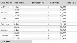
In this example, you will integrate array formulas with a car sales report.

Multi-Cell Array Formula

To start, you need to multiply the values of the array in the range C2 through D13, which is the number sold multiplied by unit price for each row. With multi-cell arrays, you can write the formula in one place and have it populate the cells you choose.

Select cells E2-E13.

Next, type the following in the formula bar:

=C2:C13*D2:D13

Press CTRL + SHIFT + ENTER.

Pressing this combination of keys will let Excel know that you are entering an array formula. Your formula will automatically be surrounded with curly braces in the formula bar as a result.

If done correctly, all cells will populate with the correct answer.

Single Cell Array Formula

Now we will calculate the total sales. Select cell B14. The following formula will add the products of “number sold” and “unit price” columns.

=SUM(C2:C13*D2:D13)

Press CTRL + SHIFT + ENTER to enter the formula. The answer will appear, and you are finished.