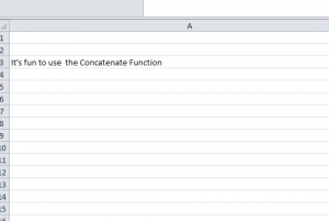
Combining several cells and any values contained within them into one cell is easy to accomplish with the Concatenate Function. This is a trick that is quick to implement. This Excel function is helpful when you need to combine cells for extended messages that are a few sentences long and don’t want to break up the words, phrases, or data in individual cells. You can make your spreadsheet look nice and neat with this easy to use formula.
How to Use the Concatenate Function in Excel
To begin, you can either use a template you have already created or download the free example template provided for you at the bottom of this screen.
After you have your spreadsheet open, then everything you need to know about the Concatenate Function is pretty much summed up with one word, ampersand (&).
First, write your message out in the individual cells. In the sample spreadsheet, the original message is located to the right of the screen. You can see how this is aesthetically displeasing when compared to the right-hand view of the message that has been combined into one cell.
To accomplish this trick, simply click inside the cell you want to start your message and use the Concatenate Function. Then, add the following formula into the function bar, once you have chosen your cell.
=B3&C3&D3&E3&F3&G3&H3
Note that the values for this formula are taken from the example spreadsheet. Remember to change these values to correspond with your own message or data. The only thing that won’t change will be the SUM at the beginning of the formula and the ampersands connecting each specified cell throughout the document.
After you have typed out the formula and hit enter, you’ll see your entire message displayed in the location you have chosen, free of any hindering cell lines.
The Concatenate function is your best friend when it comes to making your spreadsheet clear, simple, and professional-looking.
Download: Concatenate Function Sample
Check out this offer while you wait!

