Using the COUNT function to create ranges between certain numbers is a great way to create lists based on prices and other criteria for your business. This useful function is the best friend of anyone looking to organize their spreadsheet lists by creating ranges. The free template file below will guide you through the steps to properly use the COUNT function for this purpose and teach you how to apply it for your own purposes later on. If you’re ready to start organizing your business or even your personal finances at home with this great tool, simply continue reading the guide below.
How to Use the COUNT Cells Between 2 Numbers Template
The best way to learn how to use Excel functions is to follow along. Click the link provided below to download the free template file directly to your computer.
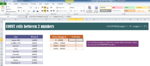
Now, the example is very simple. Let’s suppose you sell cars and you want to list the cars that fall in a certain price range on your site, making it easier for potential customers to shop for what they need.
The first column of the purple template will list the cars that you sell and the second column is the exact price of those cars.
In the orange table to the right, you have listed 3 different ranges that you want to use the COUNT function to calculate for you. The general formula that you will use for this purpose is listed below.
=COUNTIFS(range,”>=X”,range,”<=Y”) Let’s say you want to see the number of cars that fall between $0-$2000, you would enter “=COUNTIFS(Table2[Price $],”>= 0″, Table2[Price $],”<= 20000″).”
The “Range” section is taken from the orange table based on the ranges you created and the prices from the purple table as well. The “X” value would be the first number in your range and the “Y” is the maximum. The second range is just the prices from the first table as well.
Using this function, you can create an accurate range of any item quickly and efficiently.
Download: COUNT cells between 2 numbers
Check out this offer while you wait!

