

Learn how to prepend text in Excel spreadsheets easily and quickly. Using a formula to prepend text results in creating new information within a cell that is slightly altered from previously entered information. This is useful for categorizing and updating your spreadsheets. Prepend text goes before the indicated text and can used for a number of purposes. Read on to learn how to achieve this feat of Excel prowess.
Download the Prepend Text example and follow along to learn.
How to Prepend Text:
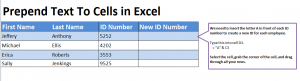
- Open up your downloaded prepend example sheet and view the four columns, one empty, and four rows. Your goal is to fill in that last row with this formula’s results.
- Choose the cell you want your prepend added – D3 here – and enter the following formula: = “A” & C3
- The formula will result in cell D3 being populated with “A5252”.
- To use this formula to the remaining cells in the row, drag down from D3 and the rest will be finished automatically.
Why should I use Prepend Text?
- Alphabetical organization is made easy with this formula. simply preface rows with A, B, C, etc to achieve this.
- It’s much quicker than entering each cell manually.
- Keep Excel updated easily with this formula because of its drag feature. Apply mass changes with a click of your mouse.
Tips for Success: Spend time in the example trying different formula variations before going into your intended Excel document. Change “A” in the formula to “Terminated”, “In Progress”, or other statuses to get a feel for how to split up groups.
Check out this offer while you wait!