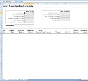
Loan Calculation – Building An Amortization Table in Excel

Loan Calculation – Building An Amortization Table in Excel

Knowing how to build an amortization table will give you a good handle on your monthly payment for a loan and how much you will pay in interest over the course of your loan. I use amortization tables a lot in both business and in my personal life. For business, I usually use it to determine a monthly payment or determine the actual interest rate of a loan. Often, a loan will include a monthly processing fee or a service fee upfront – really just another form of interest, but if you are comparing two loans, you need to know what your true cost of capital is. In personal use, I use an amortization table to determine what my mortgage interest is for the purposes of calculating my estimated taxes. I also use it for determining what the payment will be on a car loan based on different loan terms, for instance.

Information you need:

• Loan amount (example: $200,000)
• Interest rate (example: 6%)
• Loan term in months (for this example, we are saying 36 months)

1. Open Excel, in cell A-1, type ‘Interest.’
2. In cell B-1, type your annual interest rate.
3. In cell A-2, type ‘Term’, in B-2, type ‘Payment’, in C-2, type ‘Interest’, in D-2, type ‘Principal’, in E-2, type ‘Outstanding’.
4. In cell E-3, type your total loan amount.
5. In cell A-4, type ‘1’.
6. In cell A-5, type ‘=A4+1’.
7. Copy and paste into cells in the A column below A-5 until you get A-39 (or so that the number in the last cell equals the number of months of your loan).
8. In cell B-4, type a reasonable number for your payment, 1,000 for every $100,000 in borrowed money will work fine.
9. In cell C-4, type “=E3*$B$1/12”.
10. In cell D-4, type “=B4-C4”.
11. In cell E-4, type “=E3-D4”.
12. In cell B-5, type “=B4”.
13. Copy cells C-4 through E-4 into cells C-5 through E-5.
14. Copy cells B-5 through E-5, and paste them in every row from row 6 to the row 39.
15. Select cell E-39.
16. Select ‘Goal Seek…” from the Tools menu.
17. In ‘Set cell:’, it should say ‘E39’.
18. In ‘To value:’, type in ‘0’.
19. In ‘By changing cell:’, type ‘B4’.
20. Hit OK.

This will give you the exact payment and monthly interest and principal payments for your loan. Remember if you change the term of your loan, the places where I have put ‘E39’ will have to be changed to the row where your last term month is.