Applying Conditional Formatting in Excel

Download the example Excel sheet to follow along

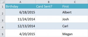
Applying conditional formatting to an Excel file is a handy process to know. The example is showing how the Excel program tracks birthdays of clients, and notes when a date has a passed. As a triggering action, once a date has passed, the formula will mark the “Card Sent” cell with a “yes”.

Here is how you create this Excel sheet. Use the example you downloaded to learn.

Start by selecting cells A2 through A5.

Click “Conditional Formatting” in the Excel Ribbon Tool.

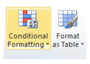
Next, click “New Rule” from the drop down menu.

A dialog box will pop up. Select “Use a formula to determine which cells to format.”

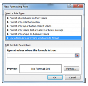
In this example, enter in the format value textbox “=a2>TODAY()” and click the “Format” button.

In the top “Font” tab, select red and make the font bold. Press OK, then press OK again to hide the dialog box if it is still open.

The cell text will be bold and red if the birthday is in the future.

IF statements

Continuing through the example, go in cell b2 and enter the following:

=IF(A2<TODAY(),”Y”,””)

This will indicate if the day is in the past. If so, the cell will be marked with as “Y” for yes, which will tell you if you sent the person a card for their birthday.

Lastly, drag the formula through B5 using the fill handle so all the cells in that column have the same formula. You’re finished! Use this conditional formatting exercise for any Excel sheets that you want automatically updated.