COUNT Matches Between Columns

If you’re tracking multiple lists of items and what to see if there are any matches across multiple columns, it can be quite the pain to search through them all. The COUNT function can find those matches for you instantly. All you need to do is learn one simple function to save yourself hours of frustration and worry. The free template provided for you below, along with this guide, will show you how to use this great Excel function in no time at all. If you’re interested in using this function for your own use, download the template and follow along with this free guide.

How to Use the COUNT Matches Between Columns Template

To download the free template file and follow along with this guide, just click the link provided for you below.

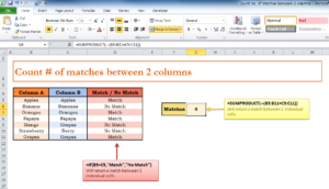
Now, when you have the document opened, there will be three columns with data. The first two columns list different fruit and the last column shows the number of matches in those columns. Using this COUNT function, you will be able to calculate the number of matches in two columns (as shown in the yellow table to the right).

The general form of this function will look like this:

=SUMPRODUCT(–(range1=range2))

Now, it’s up to you to take your variables and apply them to the basic function above. You will need two different ranges to complete the formula.

Sticking the example of fruit in the template, you would enter the following modified function into a new cell to get the same result as the “Matches” table.

=SUMPRODUCT(–(B5:B11=C5:C11))

You can see that the ranges for column A and B replace “range1” and “range2” within the basic function. This just specifies that you want to find matches within these two columns. That’s all there is to it. Once you have entered the formula, you will display the same value seen in the yellow table.

Download: Count no. of matches between 2 columns