

Learn the Excel Left Formula to grab characters from the left part of a cell and put that data into another cell. Use this function to simplify or abbreviate data that is already in your spreadsheet to help you search, convert, or organize your data in an easier way. The Excel Left function is easy to input and experiment with and use in your own spreadsheets.
Download the Example page and follow along with our guide.
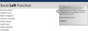
Open the example and you will see a simple one page sheet with one column filled with names. This is where you will pull data from for the B column. The left function will pull data from whatever cell you indicate, and will take the amount of characters that you choose. To try this out, go to cell B3 and enter:
=left(A3,5)
The A3 is where you want the data taken from, and the “5” is how many characters, starting from the far left character, taken. The result for this will be “Micha”.
To apply this same formula to all the names, grab the corner cell B3 and drag it down to B10. This will take the first 5 characters from each of those names and put them into their corresponding B column cells. You can go back to any cell that was auto-filled and change the formula if you want to, or leave it as is.
Learn more about Excel in our tutorials.
Check out this offer while you wait!