

Another exciting feature of Excel is its ability to be customized to your every desire and aesthetic. You can change elements such as colors, fonts, borders, and alignment.
Download the example Formatting Data spreadsheet to follow along
Formatting Color, Size, and Fonts
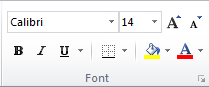
Start with changing colors, which is helpful in color-coding cells and organizing visual Excel files. In the example file, select cell “A2” and then move to the toolbar up top. The image of the bucket pouring a yellow color is the Highlighting tool. Click it, choose a color, and your A2 cell will be highlighted. The bottom next to it with an “A” and a red bar will change the actual text color.
Use this same process to change fonts, sizing and more from the editing toolbar above.
Formatting Numbers
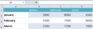
You can easily change how numbers are read and represented in Excel. In the example spreadsheet, highlight the cells with number amounts. Right click and choose “Format Cells.”
In the dialog box that pops up, select the category “Currency.”
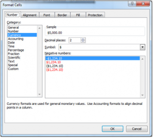
The options, such as Currency, will alter the numbers to represent what you need such as dates and fractions. All you have to do is enter the general number and use the “Format Cells” box to change them.
How to use the Fill Handle
The fill handle will let you take formatting and formulas from other cells and copy them to new ones. Using the same spreadsheet, follow the steps below to automatically fill in the months following March.
Click on March in cell A4. Hover the mouse over the bottom right corner that has a square in it, and wait for a small cross to appear.
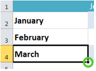
Drag the small black cross downwards on the spreadsheet to around row 13. This will make all the months of the rest of the year automatically fill in.
Check out this offer while you wait!