Using conditional formatting, you can highlight cells based on their contents. You can do this with multiple “if statements”, but Excel makes it easier with conditional formatting.
Download the example to follow along.
This example includes a gradebook. The goal is to highlight grades that are 90% and higher.
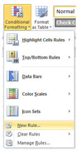
To start, make sure you have selected the range with the values you need. In the Ribbon’s Home tab, select Conditional Formatting and click New Rule.

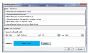
In the dialog box that follows, select “Format only cells that contain”.
Then in the boxes near the bottom of the dialog, you will see the title “Format only cells with” and four dropdowns. Select the following options:
Cell value, between, 90 and 100.
Click the Format button and select a fill color.

Press OK.
Your spreadsheet will produce cells with a different color background based on what you have previously chosen containing scores that are 90% and above. You’re finished!

Check out this offer while you wait!

