

Excel will always have a default size associated with the charts you want to use. Sometimes, this can be somewhat frustrating, as the sizes are often too small to give the impression you want to make in a presentation or project. Learning to move and resize charts in Excel is the best way to get your spreadsheet looking just the way you want. Moving and Resizing are some of the easiest tricks you can do in Excel. Read the list of instructions below to learn how to do it!
How to Move Charts in Excel
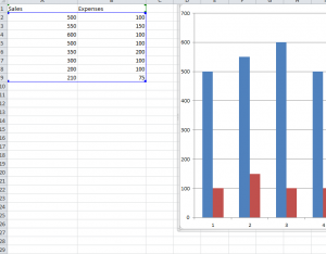
Start by creating your data in a table. The free example spreadsheet is available to download below for you to follow along.
Once you have created your data points, like the table those featured to the left of the example spreadsheet, continue to insert a graph of your choosing. A table should appear, just like the one featured in the sample.
To move the graph within the document, simply place your mouse inside the graph. Your cursor should change to multiple arrows pointing in the 4 cardinal directions. From this point, you can simply click in the blank white space of your graph and move it anywhere you wish, and then drop the graph where you want it to be.
If you want to move your graph to another worksheet, you can easily copy and paste it into your new document.
How to Resize Charts in Excel
To resize you graph in Excel, start by moving your cursor over one of the corner of your graph until the cursor changes to a white double-sided arrow icon.
From this point, you can easily click and drag the graph to change the size until it’s exactly the way you want. Moving and resizing charts in Excel has never been easier, just use the methods above to create your perfect chart.
Download: Moving and Resizing Charts in Excel
Check out this offer while you wait!