

Excel has the ability to customize rows and columns through dropdown menus. With Dropdown lists, you have access to many different data choices for output within a cell.
Download the Dropdown List example page to follow along.
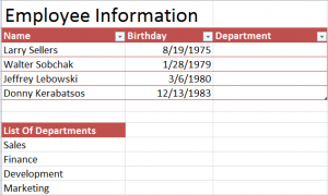
In our example, we will show how to easily assign an employee to a department using dropdown lists.
How to create a dropdown list in Excel
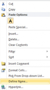
Select the “List of Departments” in the example and drag to have A9 through A13 highlighted together. Then right click and choose “Define Name” from the list that appears.
A new box called “New Name” will appear, give the list title a descriptive name like Departments.
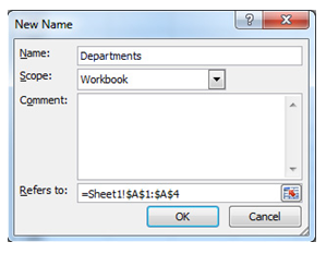
Press Enter. Now you have created a list of the departments in Excel. From here, all that is needed is to tell Excel where to insert the list in the rest of the spreadsheet.
Start by highlighting cells C3 through C6.
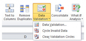
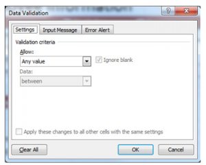
Click the “Data” tab in the top Ribbon bar and select “Data Validation”. From the dropdown list, pick the “Data Validation” option.
In the Data Validation dialog box, make sure you’re on the “Settings” tab. In the dropdown under “Allow”, select List. More options will then appear in the dialog box. Click the text box located under “Source”.
Type in “=Departments” (without quotations) or the name you came up with earlier for the list.
If you wish to customize messages for the dropdown, there are two tabs in the dialog called “Input Message” and “Error Alert” for you to use.
When you’re finished, press enter.
Under “Employee Information”, go to the empty “Department” cell next to an employee’s name and click the empty cell. A dropdown arrow will appear and show the options for each department to assign to that employee. You’re finished!
Check out this offer while you wait!