

The VLOOKUP function allows a user to search the very first column in a cell range and return data from a cell in the same row of that range.
Download the example to follow along and learn how to use this function.
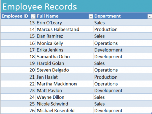
In our example, the VLOOKUP function will be used to return the full name or department by using the employee ID in the formula.
Syntax
VLOOKUP(lookup_value, table_array, col_index_num, [range_lookup])
Lookup_value – the value to search for
Table_array – the range of cells that contains the data.
Col_index_num – the number of the column in table_array that we want a matching value from.
Range_lookup – (optional) determines if an exact match or an approximate result can be returned
VLOOKUP in Action
For this example, we want to find out the full name of employee number 22 in our employee database.
In the example spreadsheet, select cell A18.
This is where you will start building the VLOOKUP function.
Since we know what the value (employee number) to search for in the first column, enter:
=VLOOKUP(22,
Then, input the range of the data to search through.
=VLOOKUP(22,a3:c16,
Next, choose the number of the column that has the data we’re looking for. “Full name” is column 2.
=VLOOKUP(22,a3:c16,2,
And we need an exact match on the lookup.
=VLOOKUP(22,a3:c16,2, FALSE)
Now that we have our formula, enter it in cell A18. The result should be Martha Mackinnon.
Check out this offer while you wait!